by Rachel Street
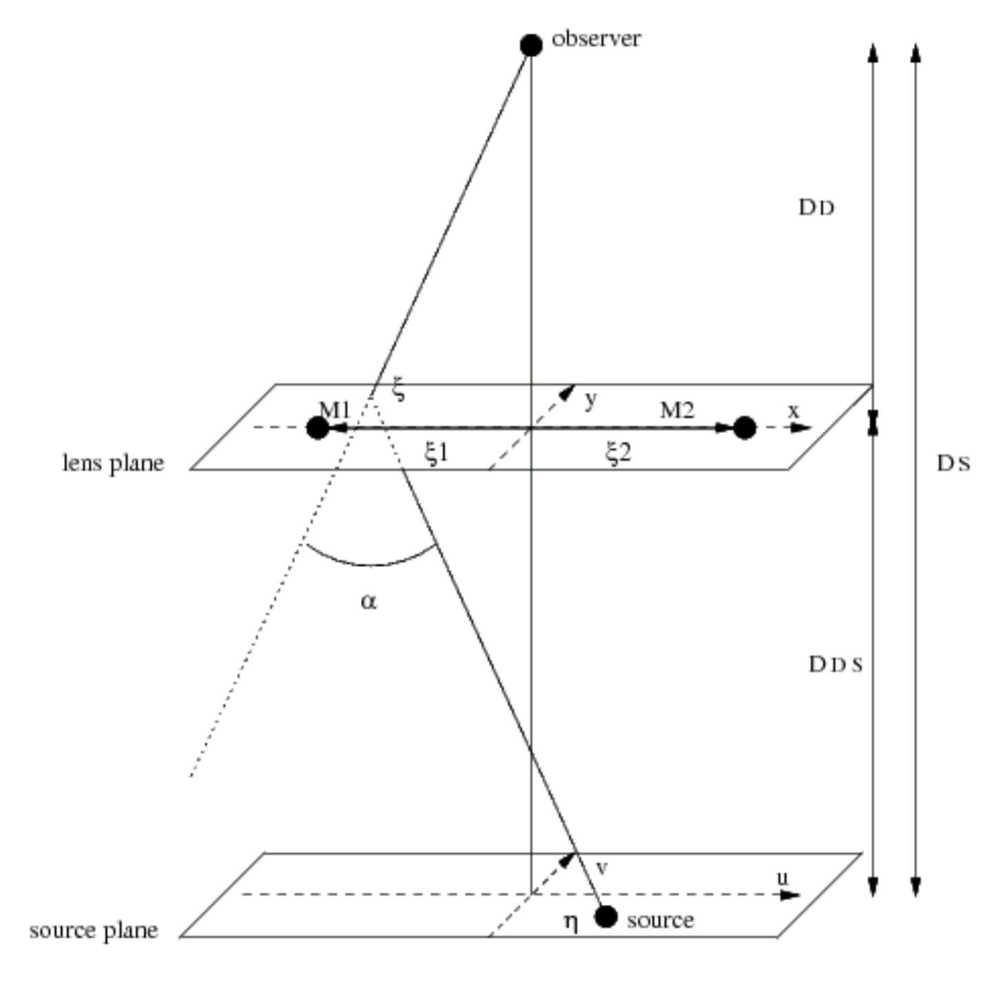
A binary lens consists of two masses, M1 & M2. The lens plane coordinate system (x,y) is arranged so that the x-axis passes through the projection of the masses onto the lens plane, with the origin at the central point between the two lens masses (Fig. 11). Both are considered to be at distance DL from the observer, their separation being relatively small.
The source plane is described by coordinate system (u,ν), which has its origin at the point where the optical axis intersects the plane.
Each mass deflects a light ray from the source by angle α = 4GM/c2b. The total deflection is then the vector sum of the deflections by each of the individual masses. Taking an example ray which intersects the lens plane at ξ = (x1, y1), the total deflection in the general case for a lens with i = 1 - n masses is given by:
| $$\bar{\alpha}(\bar{\xi}) = \sum_{i}\left( \frac{4GM_{i}}{c^{2}}\frac{\bar{\xi} - \bar{\xi_{i}}}{|\bar{\xi} - \bar{\xi_{i}}|^{2}}\right),$$ | [37] |
For a binary lens this becomes:
| $$\bar{\alpha}(\bar{\xi}) = \frac{4GM_{1}}{c^{2}}\frac{\bar{\xi} - \bar{\xi_{1}}}{|\bar{\xi} - \bar{\xi_{1}}|^{2}} + \frac{4GM_{2}}{c^{2}}\frac{\bar{\xi} - \bar{\xi_{2}}}{|\bar{\xi} - \bar{\xi_{2}}|^{2}},$$ | [38] |
where ξ̄1,2 are the vector positions of the projection points of masses M1,2 in the lens plane geometry.
We now write the lens equation in a form relating the lightray origin in the source plane (η(u,ν)) to the total deflection angle:
| $$\bar{\eta} = \bar{\xi}\frac{D_{S}}{D_{L}} - D_{LS}\bar{\alpha}(\bar{\xi}),$$ | [39] |
By substituting Eqn. 38 into 39 we get:
| $$\frac{\bar{\eta}}{D_{S}} = \frac{\bar{\xi}}{D_{L}} - \frac{4GM_{1}}{c^{2}}\frac{\bar{\xi} - \bar{\xi_{1}}}{|\bar{\xi} - \bar{\xi_{1}}|^{2}}\frac{D_{LS}}{D_{S}} - \frac{4GM_{2}}{c^{2}}\frac{\bar{\xi} - \bar{\xi_{2}}}{|\bar{\xi} - \bar{\xi_{2}}|^{2}}\frac{D_{LS}}{D_{S}},$$ | [40] |
This is simplified by declaring:
| $$\bar{w}(u,\nu) = \frac{\bar{\eta}}{D_{S}},$$ | |
| $$\bar{z}(x,y) = \frac{\bar{\xi}}{D_{L}},$$ | |
| $$m_{i} = \frac{4GM_{i}D_{LS}D_{L}}{c^{2}D_{S}},$$ | [40] |
and we arrive at:
| $$\bar{w} = \bar{z} - m_{1}\frac{\bar{z} - \bar{z_{1}}}{|\bar{z} - \bar{z_{1}}|^{2}} - m_{2}\frac{\bar{z} - \bar{z_{1}}}{|\bar{z} - \bar{z_{1}}|^{2}},$$ | [41] |
As before, this represents a mapping between the source and lens planes. A lightray from point w̄(u,ν) in the source plane will hit the lens plane at z̄(x,y). The inverse problem, extracting the locations of the source images in the lens plane geometry requires complex root-finding techniques explored in detail by Schneider & Weiss (1986). In complex notation, Eqn. 41 becomes:
| $$w = z - m_{1}\frac{1}{\bar{z} - \bar{z_{1}}} - m_{2}\frac{1}{\bar{z} - \bar{z_{2}}},$$ | [42] |
where w, z are complex numbers:
| $$w = u + i\nu,$$ | |
| $$z = x = iy,$$ | [43] |
and z̄ is the complex conjugate of z.
To find the number and locations of the source images produced we need to produce an expression for z in terms of w - the inverse of the lens equation. The complex conjugate of Eqn. 42 is:
| $$\bar{w} = \bar{z} - m_{1}\frac{1}{z - z_{1}} - m_{2}\frac{1}{z - z_{2}}.$$ | [44] |
Solving this expression for z̄ and substituting into Eqn. 42, we get:
| $$z = w + \sum_{i=1,2}m_{i}\left[\bar{w} - \bar{z_{i}} + \sum_{k=1,2}m_{k}(z - z_{k})^{-1}\right]^{-1}.$$ | [45] |
This expression generates a polynomial equation in z of order (n2 + 1), where n is the number of lensing masses. Therefore, for a binary lens, there are up to 5 solutions, of which either 3 or 5 may be real, depending on the lens-source projected separation (see later discussion, and references).
Following similar arguments used to derive the amplification of a single-mass lens, that for a binary lens is, as before, the inverse of the area distortion of the lens mapping (compare with Eqn. 16):
| $$A = \left| det \frac{\partial\bar{w}(u,\nu)}{\partial\bar{z}(x,y)} \right|^{-1},$$ | [46] |
To derive an expression for this we need the 'gradient' of a vector function, or the matrix of first-order partial derivatives, known as the Jacobian matrix, which may be written:
| $$J = \begin{bmatrix} \frac{\partial u}{\partial x} & \frac{\partial u}{\partial y} \\ \frac{\partial \nu}{\partial x} & \frac{\partial \nu}{\partial y} \end{bmatrix}$$ | |
| $$J = \left| \frac{\partial w}{\partial z} \right|^{2} - \left|\frac{\partial w}{\partial z}\right|^{2},$$ | [47] |
which for n lensing bodies is:
| $$J = 1 - \left[ \sum_{n} m_{n}(\bar{z} - \bar{z_{n}})^{-2}\right]^{2} = 1 - (\bar{\kappa})^{2},$$ | [48] |
and for a binary lens is:
| $$J = 1 - \left( \frac{m_{1}}{(\bar{z} - \bar{z_{1}})^{2}} + \frac{m_{2}}{(\bar{z} - \bar{z_{2}})^{2}}\right)^{2},$$ | [48] |
The inverse Jacobian matrix elements are:
| $$\frac{\partial z}{\partial w} = \frac{1}{J},$$ | |
| $$\frac{\partial z}{\partial \bar{w}} = -\frac{\bar{\kappa}}{J},$$ | [49] |
The total amplification is given by the sum of the absolute amplification of each image i:
| $$A = \sum_{i=1}^{n}A_{i} = \sum_{i=1}^{n}|\det J|^{-1}.$$ | [50] |
Mathematically, the nature of this solution has a curious feature. As the source moves behind the binary lens, there are certain positions in the source plane for which the resulting Jacobian determinant drops to zero:
| $$\det J = 0.$$ | [51] |
These positions form graceful curves, known as 'critical curves'.
Theoretically, as the source crosses the critical curve, the amplification becomes inifinite, according to Eqn. 50. In reality, finite source effects curtail the amplification to merely 'high', but these situations can still result in very dramatic brightenings of the source by several magnitudes.
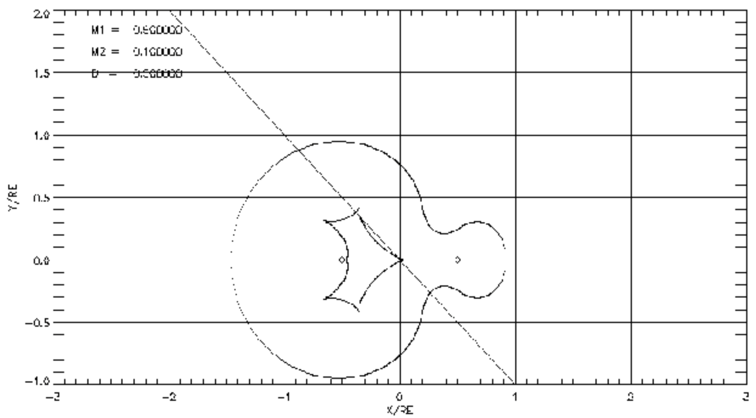
Applying the lens equation, the positions of the critical curve in the source plane can be mapped into the lens plane geometry - resulting in generally spiky curves known as 'caustics'. Both are illustrated in Fig. 12.
|
(Top) Lens-plane geometry view of a binary lens of unequal masses (normalized so that M<sub>1</sub> + M<sub>2</sub> equals 1). The straight line indicates the source's relative motion during the event. The curved loop around both masses is the critical curve in the source plane; the spiky central region between the masses represents the caustic. (Bottom) The event lightcurve resulting from this configuration.Y. Tsapras |
The number of images changes as the source moves across the caustic curve. Outside it, there are three images; one outside the critical curve and two inside it, usually close to one of the masses. Whereas when the source lies within the region defined by the caustic, two more images exist, one inside and one outside the critical curve. Its interesting to bear in mind that the caustic curve represents the maximum amplification, and the amplification within the caustic actually drops. For wide binary lenses, the amplification mid-caustic can drop back almost to baseline.
The expressions derived here depend on the ratio, q, of the masses of the lensing bodies and their positions in the lens plane. These factors dictate the shape and extent of the caustics and a wide variety of shapes are possible. The source can also take any trajectory, relative to the lens geometry. A wide range of lightcurves can result, but one common feature is a 'double-peak' structure - the first peak caused by the source crossing into the caustic region, the second caused by it exiting the caustic. Depending on the size of the caustic, the trajectory and relative velocity, the peaks can be hours or days apart.
Notice though, that a binary lens of any q will produce caustics. Therefore, if the source has a favourable relative trajectory, even an extreme mass ratio binary like a planetary system will produce a detectable amplification. This makes microlensing uniquely sensitive to even low mass planetary companions. However, the caustic region for low mass ratio lenses is generally smaller, so the crossing time (the duration of the anomaly) is usually shorter (depending on the velocities of source and lens) and requires better lightcurve cadence to detect. The probability of the source trajectory crossing the caustic is also smaller, but this is factor compensated for by surveys covering large numbers of stars.