by Rachel Street
Continuing to explore complications which can cause microlensing events to deviate from purely PSPL models, we will now look at a more data-orientated issue which is nevertheless related to parallax because it's affects can mimic a parallax signature; the two are degenerate and need to be considered carefully. This issue is blending.
Assumption No. 2: That the image of the lensed source in our CCD frames is always isolated and the flux from it can always be measured independently from all neighboring stars.
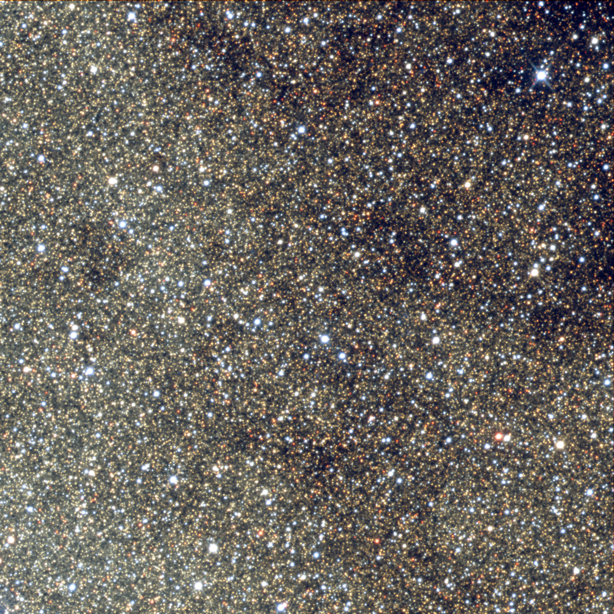
Microlensing is an intrinsically rare phenomenon, due to the precise alignment required between observer, lens and source. To detect these events in significant numbers, all surveys to date have concentrated their observations in very dense starfields such as the Galactic Bulge and Magallenic Clouds. The resulting CCD images are very crowded and its rare to have star which is entirely isolated from its neighbors.
Although we don't resolve the disk of the stars in these observations - they remain points of light - the light from each star in the frame is spread over a circle of pixels due to diffraction at the telescope aperture. This shape of this circle is described by the star's Point Spread Function (PSF), which will have a certain Full Width Half Maximum (FWHM) depending on the telescope and seeing conditions at the time. The instrument detects the light via an array of pixels, each of which subtends an angle on sky (the pixel scale) which is specific to that camera and telescope. If the PSFs of neighboring stars overlap, they are said to be blended. These neighbors are probably not physically associated with the target; they could be at any distance, but lie at a close angular separation from our line of sight.
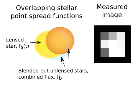
Blending results in light from the neighbors contaminating the flux measurement of the lensed star, fs. Whereas for an isolated lensed star, the flux at a given time t, f(t) is given by:
| $$f(t) = f_{s}(t)A(u(t))$$ | [29] |
in practise what we actually measure is more like:
| $$f(t) = f_{s}(t)A(u(t)) + f_{b}$$ | [30] |
where fb(t) is the additional flux from all overlapping neighbors. This is heavily time-dependant: for instance, if the seeing suddenly worsens during observations, the PSF FWHM expands and fb abruptly increases.
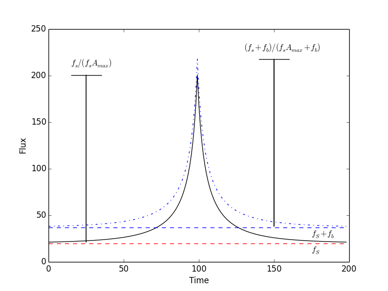
The figure above shows the affect of blending on a microlensing event. Overall, the additional flux can "dilute" the measured amplitude, and make tE appear shorter, leading to a mis-estimation of the lens parameters. As this can be a symmetrical change in the lightcurve, it can mimic the affects of the parallax component πE,⊥.
Multiple sets of observations from different instruments can help here. As each one may come from telescopes of very different aperture, fs, even unblended, will still differ between datasets just as fb, so we consider both as functions of time for each dataset, k (with Nk datapoints), in turn:
| $$f_{k}(t) = f_{s,k}(t)A(u(t)) + f_{b,k}$$ | [31] |
Of course, they’re all observing the same event, so A(u(t)) relates the datasets together.
We begin by adopting initial typical values for the physical event parameters, to derive a starting model A(u(t)). Eqn. 31 gives us a model for the flux measured from each dataset, fm,k(t), with measurement errors, σm,k(t). We can test how well the model fits with a χ2 test:
| $$\chi^{2} = \frac{\sum_{i} \left( \frac{f_{m,k}(t) - f_{k}(t)}{\sigma_{m,k}(t)} \right)^{2}}{N_{k} - N_{par}}$$ | [32] |
where Npar is the number of fitted parameters.
Differentiating this expression with respect to each variable in turn and equating it to zero, we can derive a set of simultaneous equations which can be used to infer fs,k, fb,k for each dataset, for the given amplification model.
Given this set of initial blending parameters, we can now repeat this process, but this time fit for the physical parameters of the amplification model. By iterating this process, we can arrive a set of consistent parameters for both models.