by Rachel Street
Assumption No. 3: that the source can be treated as a point source of light. Of course we know that stars have a physical extent, but generally in astronomy its pretty safe to treat them as point sources given their enormous distances! But microlensing is an extraordinarily sensitive technique and even the radius of a star almost half way across the Galaxy can have a measureable affect.
In considering non-point sources, it is helpful to introduce the use of complex- number notation, since this makes it more natural to introduce two-dimensional vectors. For this reason, much of the following theory was originally explored in the context of lensed quasars and other large-scale masses.
The lensing can be thought of as a 'mapping' of the coordinate system in the lens plane (x,y, centered on the lens) to that of the source (ξ,η), in the sense that it describes the offsets (θ1,2) of the images of the source in terms of the lens characteristics and the angular separation between lens and source(α).
Here we introduce complex notation in order to parameterize the lens equation:
| $$\zeta = \xi + i\eta$$ | ||
| $$z = x + iy,$$ | [33] |
where z and ζ are normalized to the Einstein radius in the lens, source planes respectively.
The lens equation can then be re-written:
| $$\zeta - \frac{D_{S}}{D_{L}}z - D_{LS}\alpha(z,\bar{z}) = 0,$$ | [34] |
where α is the complex deflection angle α(z, z̄) = αx(x, y) + iαy(x, y) and z̄ is the complex conjugate of z.
The solutions of this form of the lens equation are then:
| $$z_{1,2} = \frac{\xi}{2}\left( 1 \pm \sqrt{1 + \frac{4}{\zeta\zeta}} \right)$$ | [35] |
See Witt 1990, Witt & Mao 1994 and Mao & Witt 1998 for a detailed introduction of this form of the lens equation and full derivation of finite-source expressions.
In this notation a single, circular source of finite radius r can be described as:
| $$\zeta(\phi) = \zeta_{0} + re^{i\phi},$$ | [36] |
where φ = θ-2π and ζ0 is the (parameterized) impact parameter. This is simply substituted into the solutions for the lens equations to derive the parameterized image locations:
| $$z_{1,2} = \frac{\zeta_{0}+re^{i\phi}}{2}\left[ 1 \pm \sqrt{1 + \frac{4}{\zeta_{0}^{2} + 2r\zeta_{0}\cos{\phi+r^{2}}}} \right],$$ | [37] |
The source-plane coordinate system is taken to be orientated so that ζ0 lies along the ξ-axis and so is real.
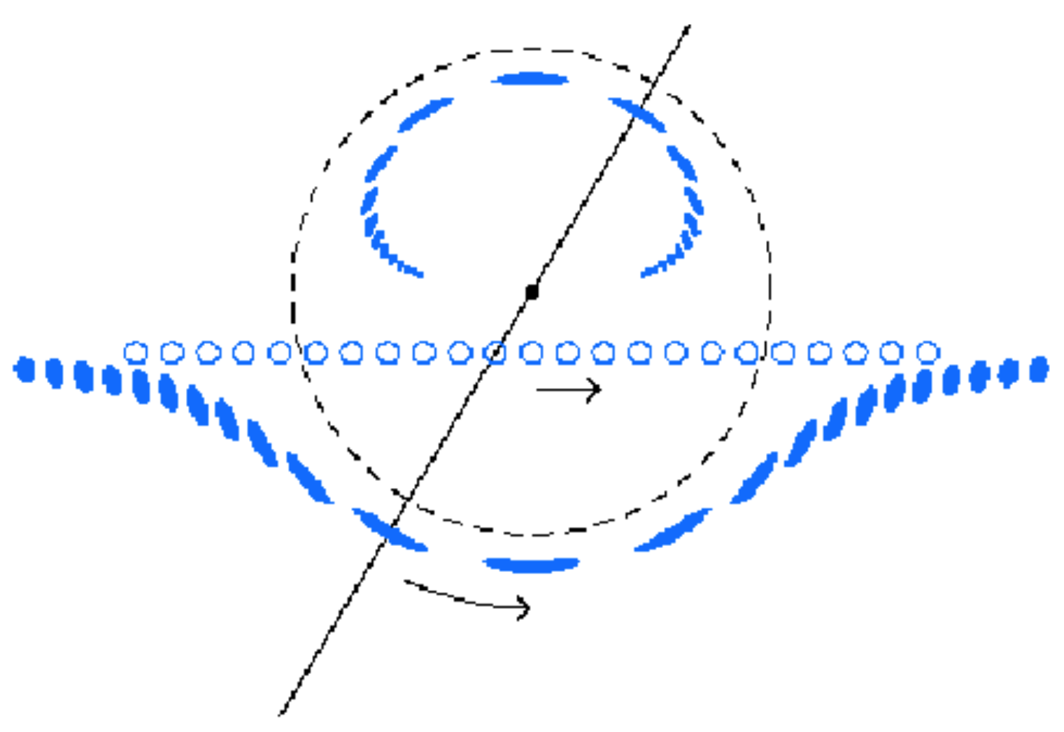
This leads to 3 catagories of images:
If ζ0 ≤ r: 2 images merge into a ring at the Einstein radius ("perfect" alignment)
If r < ζ0 << 2: 2 images form arcs
If ζ0 ≥ 2: 2 images are increasely deformed from circular with proximity to the line of sight.
As before, since surface brightness is conserved, the amplification is given by the ratio of the combined image area to that of the source. In complex notation this is given by:
| $$A_{1,2} = \frac{1}{2\pi r^{2}} \int_{0}^{2\pi} y(\phi) \frac{dx(\phi)}{d\phi},$$ | [38] |
where
| $$x(\phi) = \frac{\zeta_{0} + r\cos\phi}{2}f_{1,2}(\phi),$$ | |
| $$y(\phi) = \frac{r\sin\phi}{2}f_{1,2}(\phi),$$ | |
| $$f_{1,2}(\phi) = 1 \pm \sqrt{1 + \frac{4}{\zeta_{0}^{2} + r^{2} + 2\zeta_{0}r\cos\phi}}$$ | [39] |
Witt & Mao 1994 derived general expressions for the image amplification A1,2 and total amplification (Atot). Where ζ0 < r ("perfect" alignment along the line of sight) the images merge to form a ring, so only Atot makes physical sense. In the general case where ζ ≠ r, the full expression for A1,2 is:
| $$A_{1,2} = \pm\frac{\pi}{2} + \frac{1}{2\pi}E\left(\frac{\pi}{2},k\right)\frac{\zeta_{0}+r}{2r^{2}}\sqrt{4 + (\zeta_{0} - r)^{2}}$$ |
| $$-\frac{1}{2\pi}F\left(\frac{\pi}{2},k\right) \frac{\zeta_{0}-r}{r^{2}}{4+(\zeta_{0}^{2} - r^{2}/2}{\sqrt{4 + (\zeta_{0}-r)^{2}}}$$ |
| $$+\frac{1}{2\pi}\Pi\left(\frac{\pi}{2},n,k\right) \frac{2(\zeta_{0}-r)^{2}}{r^{2}(\zeta_{0}+r)}\frac{1+r^{2}}{\sqrt{4+(\zeta_{0}-r)^{2}}}$$ | [40] |
where E,F and Π are the first, second and third elliptic integrals defined by Gradshteyn & Ryzhik (1980) and
| $$n = \frac{4\zeta_{0}r}{(\zeta_{0}+r)^{2}},$$ | |
| $$k = \sqrt{\frac{4n}{4+(\zeta_{0}-r)^{2}}}$$ | [41] |
However, in the case where the source can be considered to be small (r → 0) but the alignment is not perfect (ζ0 ≠ 0), we recover the familiar amplification equation for a point source by summing the contributions from A1,2:
| $$A_{tot} = \frac{2+\zeta_{0}^{2}}{\zeta_{0}\sqrt{4+\zeta_{0}^{2}}}.$$ | [42] |
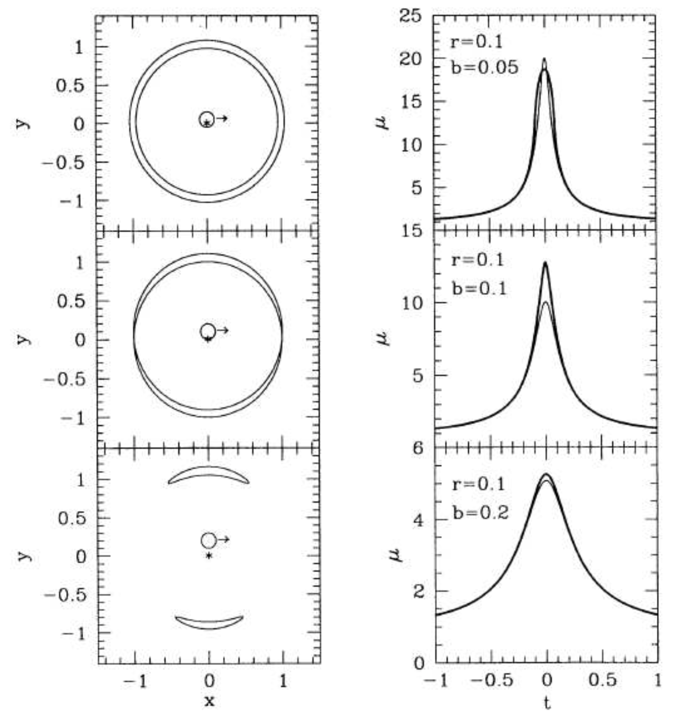
The observable effects of the finite extent of the source are illustrated in Fig. 10. The lightcurve is noticably "rounded-over" at the peak of the event in comparison with the PSPL model, and the amplitude can differ significantly. In practise this prevents real events from achieving the (theoretical) infinite amplification. These effects become significant when α ≈ θ0. This can be a problem while an event is in progress, since any deviation from the PSPL lightcurve has to be regarded as a potential planetary anomaly (ie. a binary lens). As a result, a certain amount of time is spent observing apparently anomalous events which later turn out to be due to single-object-lens.
The advantage of expressing the lens and amplification equations this way is that it makes it relatively straightforward to introduce one last consideration for a finite source – limb darkening. While the surface brightness of the source is conserved during a microlensing event, most stars don't have a constant brightness profile over the disk.
A number of well-established wavelength-dependent limb darkening relationships are available. The higher-order equations generally offer greater accuracy but are not always convenient to use. Published tables present the co-efficients for each relationship as established from observations, allowing us to look-up the appropriate coefficients for the passband of our observations. See papers by Claret et al. These coefficients have historically been denoted by uλ,1,2, somewhat confusingly in the microlensing context!
Mao & Witt (1998) implemented the limb-darkening law:
| $$\frac{I_{\lambda}(r)}{I_{\lambda}(0)} = 1 - u_{\lambda,1} - u_{\lambda,2} + u_{\lambda,1}\sqrt{1 - \frac{R_{S}^{2}}{r^{2}}} + u_{\lambda,2}\left(1 - \frac{R_{S}^{2}}{r^{2}}\right),$$ | [33] |
where Iλ(r) and Iλ(0) are the intensity of the stellar disk out to radii of r and at the center, respectively.
To find an expression for the amplification taking this into account, we break the disk of the star down into infinesimally thin 'shell' layers of radial thickness dr.
Remembering that the amplification A(r) is the ratio of the image area to that of the unlensed source, we can represent the image area of a lensed source of radius r as:
| $${\rm Area}_{\rm image}(r) = A(r)\pi r^{2},$$ | [34] |
It follows then that for a source of slightly larger radius r+dr, this area is:
| $${\rm Area}_{\rm image}(r+dr) = A(r+dr)\pi (r+dr)^{2},$$ |
The image area of the shell, Areaimage(dr), alone is then the difference between these two. The contribution of that shell to the amplification, Ashell, is given, as always, by the ratio of the shell image area Areashell(dr) and the unlensed area of the shell, 2πrdr:
| $$A_{\rm shell} = \frac{Area_{\rm image}(r+dr) - Area_{\rm image}(r)}{2 \pi r dr},$$ | |
| $$A_{\rm shall} = \frac{1}{2\pi r}{d}{dr}(\pi r^{2}A).$$ | [36] |
For each shell at radius r, the product of the area of shell's image and the intensity of the stellar disk at that radius, I(r) give the flux from the shell's image. We then extract the total flux from the images during lensing by integrating over the full radius of the source. The amplification Alimb is then the ratio of this quantity to the integral of I(r)×area over the unlensed disk:
| $$A_{\rm limb} = \frac{\int_{0}^{R_{S}} A_{\rm shell}I(r)2\pi r dr}{\int_{0}^{R_{S}} I(r)2 \pi r dr}$$ | [37] |
Ultimately, Eqn. 37 still depends on A, and when the angular separation u = α/θ0 of lens and source is large, finite source effects can be neglected.