Finite source degeneracies
Finite source effects cause measurable distortions only around the peak of a microlensing lightcurve if the angular radius of the source star is comparable with the impact parameter, u0. This can result in a number of degeneracies.
Undersampled peak degeneracy
Degeneracies can arise if this region in the lightcurve is not well sampled. A good example of this is event OGLE-2015-BLG-1482L analysed in Chung et al.(2017).
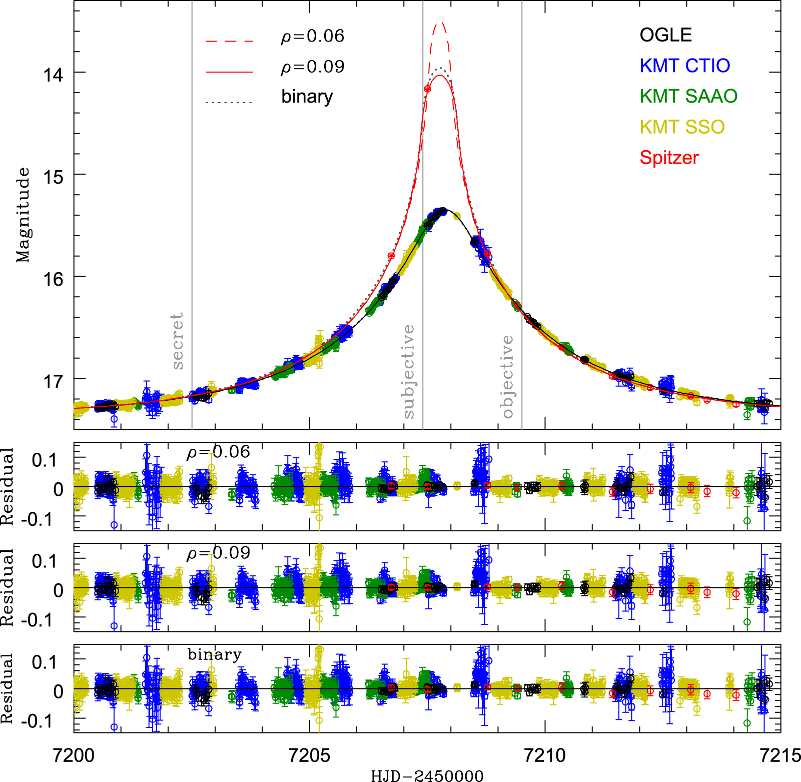
Observations were obtained from both ground-based observatories and the Spitzer Space Telescope for this event. The ground-based lightcurves are well-sampled, but Spitzer obtained ~1 observation per day. The Spitzer lightcurve was sufficient to measure the impact parameter, u, as seen from the spacecraft, as well as the source and blend fluxes, \(f_{s}, f_{b}\). But only one of the Spitzer datapoints was measurably impacted by finite source effects.
For high magnification, point-source, point-lens events, we can state that the magnification \(A_{PSPL} \approx 1/u\). Since \(f_{s}, f_{b}\) are measured, we can infer the (finite-source affected) magnification, \(A_{obs}\) at the time of the one datapoint near the peak using the measured flux F, of that point:
\[A_{obs} = \frac{F - f_{b}}{f_{s}}.\]The ratio of \(A_{obs}\) and \(A_{PSPL}\) can therefore be measured directly from the lightcurve, as shown by Gould (1994):
\[B(z) \equiv \frac{A_{obs}}{A_{PSPL}} \approx A_{obs} u,\]where \(z \equiv u/\rho\). Gould (1994) showed that B(z) reaches a maximum of \(1.34^{2}\) when z~0.91. Inverting a measurement of B(z), there is one solution of z for \(B_{obs} \lt 1\), two solutions for \(1 \lt B_{obs} \lt 1.34\) and no solutions for \(B_{obs} \gt 1.34\).
In the case of Spitzer’s lightcurve for OGLE-2015-BLG-1482L, the one datapoint near the peak has \(A_{obs}\)=1.14 and u=0.06, giving B(z)=1.15, and hence two solutions for z.
For binary events, the finite source degeneracy can result in ambiguous values of the binary separation, s, and mass radio, q. A good example of this is the event KMT-2019-BLG-1339L, analysed by Han et al.(2020).
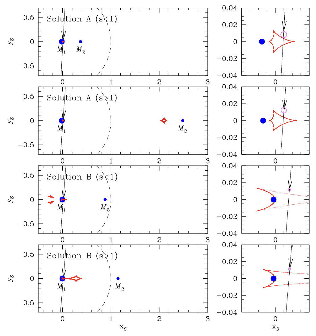
Here, different binary lens separations and mass ratios combine with different source sizes to produce similar lightcurves. These could be distinguished with higher resolution data, but this isn’t always available.
Finite/point source degeneracy
In some cases, under sampled lightcurves, particularly during short-duration anomalies, can lead to degeneracies between models with a point-source versus one with a finite value of \(\rho\).
Two real-world examples of this can be found in Poleski et al.(2017) and Han et al.(2019).
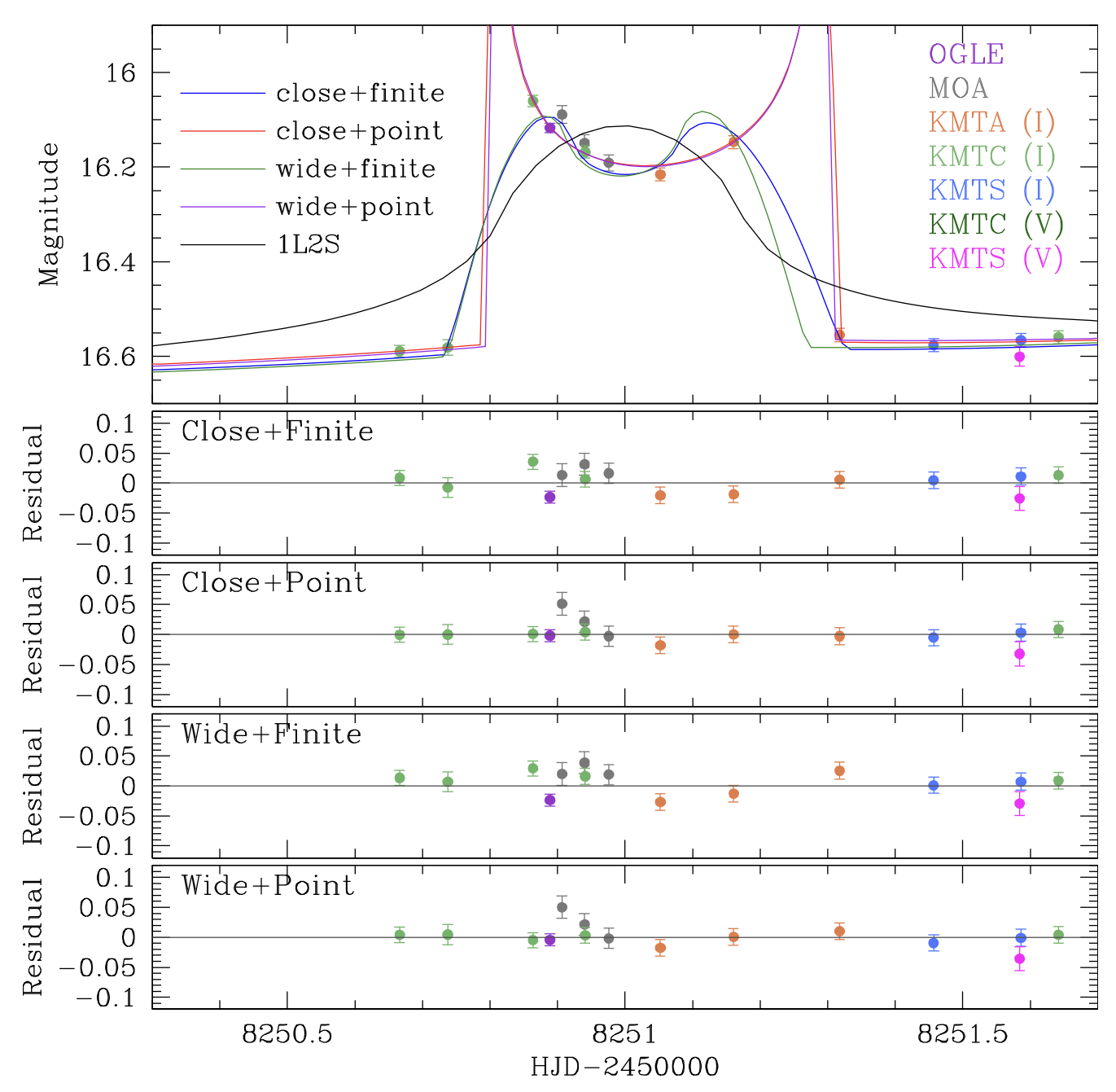
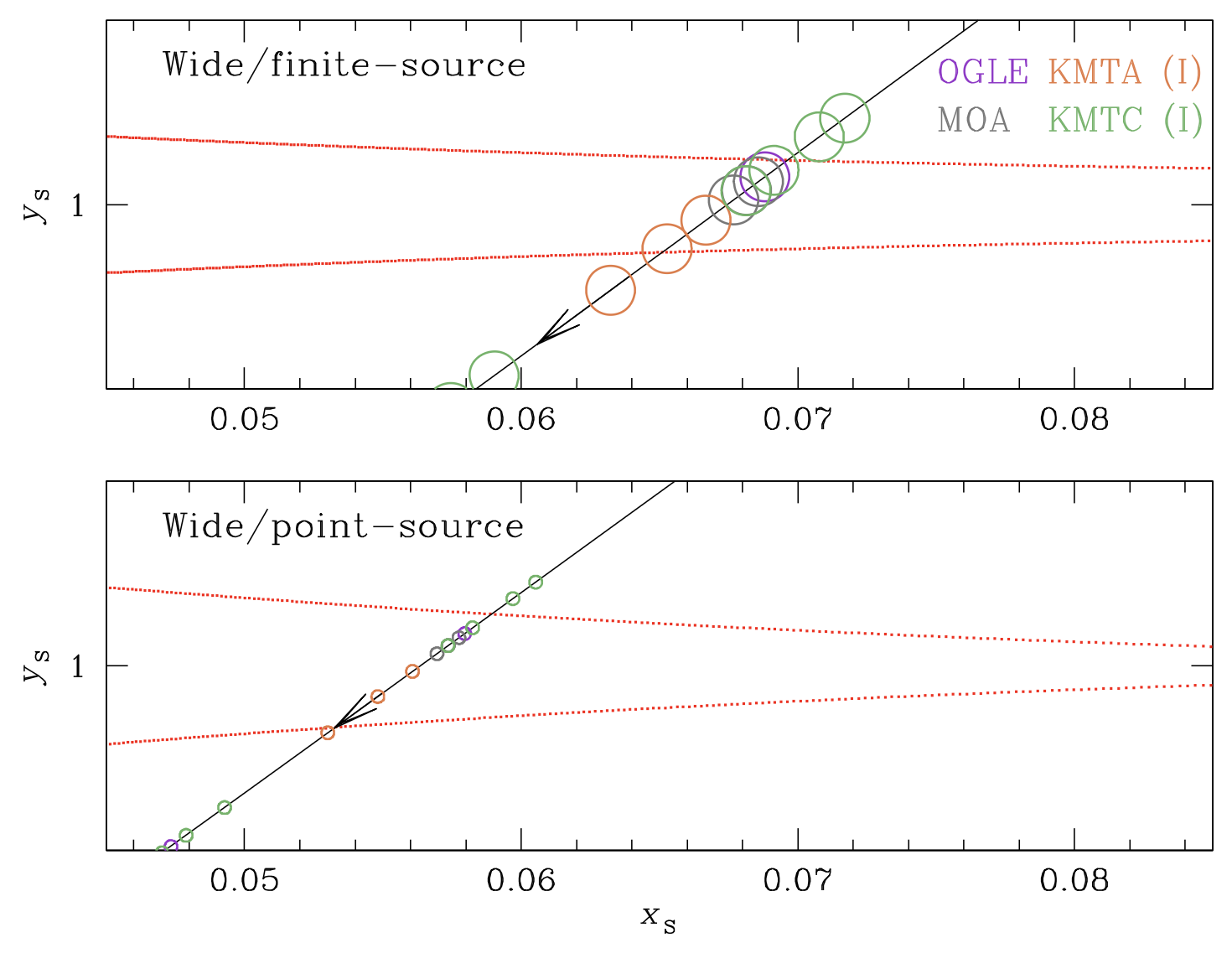
The plot above shows a zoom-in of the lens plane and caustics for the point-source and
finite-source binary models during the caustic-crossing anomaly shown in the lightcurve.
Circles mark the angular size of the source at the times when the anomaly was observed. By chance, none of the observations coincided
with the caustic entrance or exit, leaving the lightcurve anomaly’s morphology ambiguous.
As a result, the data do not constrain the value of \(\rho\).
Extreme Finite Source Events
When lensing is caused by an object of low mass, it is possible for the angular radius of the source star to exceed the angular Einstein radius of the lens. This scenario was explored in depth by Johnson et al.(2022). In these rare cases, the lens is analogous to a magnifying glass passing over the surface of the source star.
Recalling the equation of magnification for a point source,
\[A_{PS} = \frac{u^{2} + 2}{u\sqrt{u^{2} + 4}},\]the flux measured during an event is described by:
\[F(t) = F_{s}A(t) + F_{b},\]where \(F_{s}, F_{b}\) refer to the source and blend flux. Liebes (1964) showed that the magnification of a finite source deviates from the expression above when \(u_{0} \le \rho/2\), i.e. for high-magnification events. In these cases, the limb darkening of the source star must be taken into account. It is common practise in microlensing to use a linear limb darkening law, with coefficient, Γ, following a procedure introduced by Yoo et al.(2004).
When \(\rho \gg 1\), finite source effects are important for trajectories where the center of the lens passes within \(\theta_{*}\) of the center of the source. These events are modeled with 7 parameters (\(t_{0}\), \(u_{0}\), \(t_{E}\), \(\rho\), \(F_{s}\), \(F_{b}\), \(\Gamma\)), but only three quantities can be measured directly from the lightcurve: (\(t_{0}\), \(\Delta F_{max}\), \(t_{FWHM}\)).
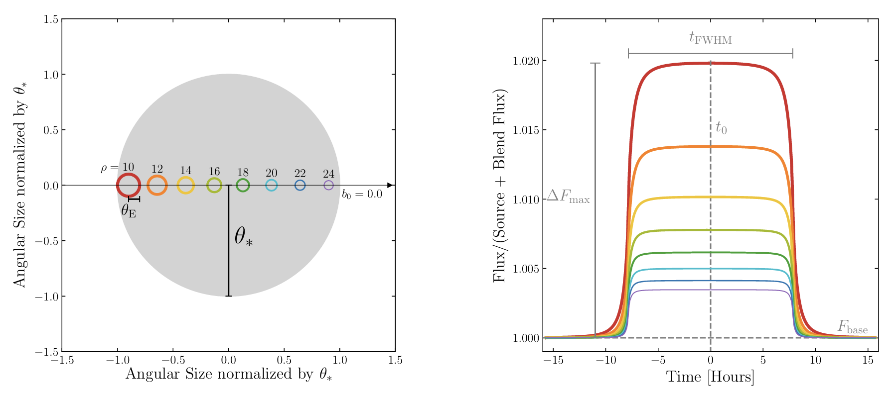
The figure above, from Johnson et al.(2022), illustrates the finite source effects produced when ρ is varied across extreme values while all other parameters remain fixed. The flux was normalized to the baseline and no blending was included. This shows that \(\Delta F_{max}\) increases as \(\rho\) decreases (i.e. the angular Einstein radius of the lens decresses). For larger values of \(\rho\), the lightcurve flattens off at the top. As a result, the duration of the event is no longer given by the source crossing time, \(t_{*}\), but is better approximated by twice the source half-chord crossing time:
\[t_{c} = \frac{\theta_{*}}{\mu_{rel}}\sqrt{1 - \left ( \frac{u_{0}}{\rho} \right )^{2} } = t_{*}\sqrt{1 - b_{0}^2} = \beta t_{*},\]where \(\beta = \sqrt{1 - b_{0}^{2}}\) and \(b_{0} = u_{0}/\rho\) is the minimum source-lens angular separation in units of \(\theta_{*}\) rather than the usual \(\theta_{E}\). This expression for the event duration is independent of \(\theta_{E}\) and hence the mass of the lens.
However, the morphology of the lightcurve also depends on the impact parameter, as demonstrated in the figure below.
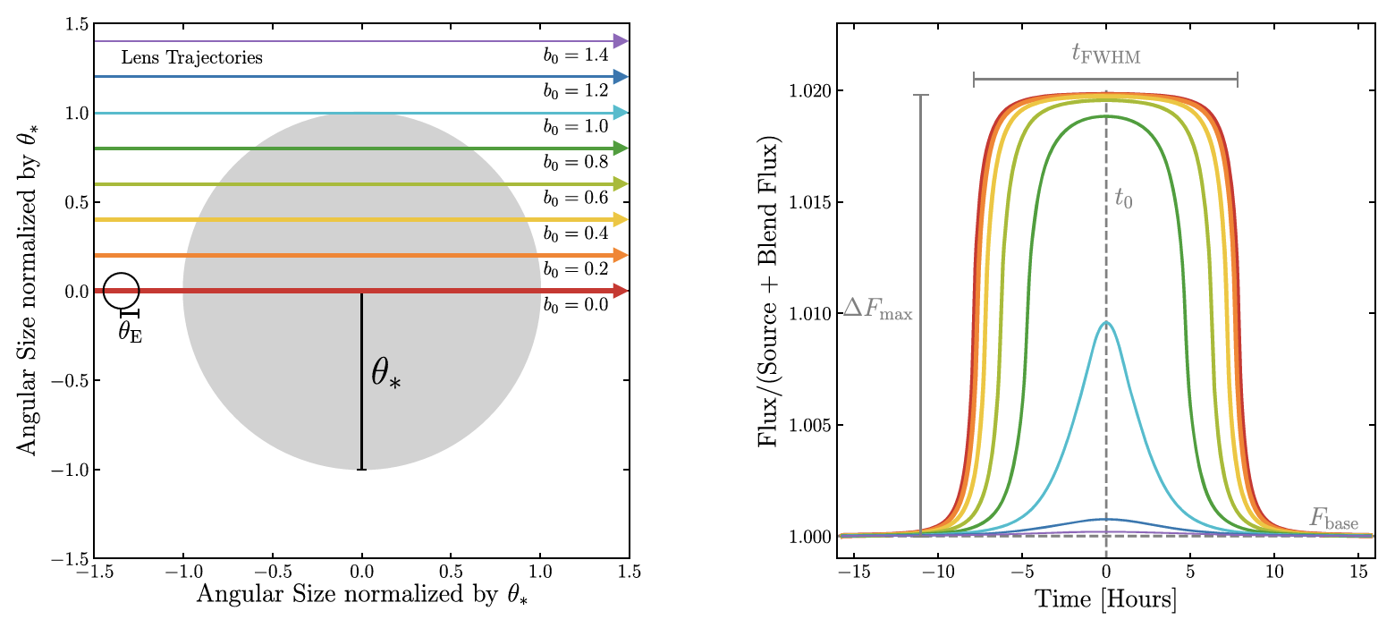
Here we see that the \(t_{FWHM}\) decreases with increasing \(b_{0}\). At low impact parameters, the same boxy lightcurve shape is seen. This has the following implications in extreme cases of finite source effects:
- the magnification during the event is effectively constant and depends only on \(\rho\). As a result, the change in flux is contant and \(\Delta F \propto 2F_{s}/\rho^{2}\);
- the timescale of the event is independent of \(\theta_{E}\) and hence of lens mass;
- the magnification is independent of duration.
The reason that the lighcurve profile has rounded corners rather than a square, top-hat profile is the finite size of the angular Einstein ring radius relative to the angular radius of the source. During the phases where the lens enters and leaves the disk of the source, the lightcurve is rounded over for a timescale, \(t_{ws} \equiv t_{E}/\beta\). This can be conveniently written as a fraction, \(f_{ws}\), of the event duration, \(t_{c}\):
\[f_{ws} \equiv \frac{t_{ws}}{t_{c}} = (\beta \rho)^{-1}.\]The duration of these “wings” and “shoulders” increases with increasing impact parameter, but also with decreasing \(\rho\).
Extreme finite source degeneracy with no limb darkening
With no limb darkening (i.e. \(\Gamma = 0\)), the maximum change in flux,
\[\Delta F_{max} = \frac{2F_{s}}{\rho^{2}}.\]It can be proven that we can factor \(F_{s}, \rho\) by an arbitrary positive constant, $\zeta$:
\[F_{s}^{\prime} = \zeta F_{s}, \rho^{\prime} = \zeta^{1/2}\rho,\]and still recover the same change in flux, meaning that in the limit of \(\rho \to \infty\), \(F_{s}\) and \(\rho\) are degenerate and
\[F_{s}^{\prime} = F_{s} \left ( \frac{\rho^{\prime}}{\rho} \right ) ^{2}.\]The same holds for the blended flux parameter, \(f_{s}\):
\[f_{s}^{\prime} = f_{s} \left ( \frac{\rho^{\prime}}{\rho} \right )^{2}.\]Similar arguments can be made for the event duration, \(t_{c} = \beta t_{*}\). Substituting \(\beta^{\prime} = \xi \beta\) and \(t_{*}^{\prime} = \xi^{-1}t_{*}\) results in equivalent chord crossing times for any arbirary positive value of \(\xi\) where \(0 \le \xi\beta \le 1\). Therefore there is a degeneracy between \(b_{0}\) and \(t_{*}\) such that:
\[t_{*}^{\prime} = t_{*}\frac{\beta}{\beta^{\prime}} = t_{*}\frac{\sqrt{1 - b_{0}^{2}}}{\sqrt{1 - b_{0}^{\prime 2}}}.\]Note that these degeneracies are only truly valid when \(\rho \to \infty\); in the more physical case where \(\rho\) is large but finite, the “shoulders” of the lightcurve will be rounded. This is important because \(f_{ws}\) is a function of \(\rho\) but not of \(F_{s}\), meaning that different values of \(\rho\) produce different lightcurve morphologies. In addition, since \(f_{ws}\) depends on \(\beta\) the shape of the lightcurve is also affected by the impact parameter. As a result, observations during these “shoulder” periods are particularly valuable.
So it is possible to substitute the four observable parameters factored by a constant, \(\eta\) into the expressions above for \(\Delta F_{max}, t_{c}\) and \(f_{ws}\):
\[F_{s}^{\prime} = \eta F_{s}, \rho^{\prime} = \eta^{1/2} \rho, \beta^{\prime} = \eta^{-1/4}\beta, t_{*}^{\prime} = \eta^{1/4}t_{*},\]and recover the same values for those parameters, meaning that the lightcurves are extremely similar.
Extreme finite source degeneracy including limb darkening
Of course, in reality stars exhibit limb darkening. For extreme finite source events, this means that the morphology of the lightcurve depends not only on \(\rho\) but also on \(\Gamma\). Since limb darkening relations themselves are a function of radius from the center of the source, this introduces a dependence on the impact parameter. It matters where the chord of the lens’ trajectory crosses the disk of the source.
Using a linear limb darkening law, the surface brightness of the source can be described as:
\[S(b(t)) = \left [ 1 - \Gamma \left ( 1 - \frac{3}{2} \sqrt{1 - b^{2}} \right ) \right ],\]This expression can be parameterized and used to describe the difference in flux as a function of time in the presence of limb darkening:
\[\Delta F(t) = \frac{2F_{s}(1-\Gamma)}{\rho^{2}} \times \left ( 1 + \frac{3\Gamma\beta}{2(1-\Gamma)} T_{c}(t) \right ) H(1 - |\tau_{c}|),\]where the half-chord crossing time, \(\tau_{c} = (t - t_{0})/t_{c} = \tau_{*}/\beta,\) and H is a Heaviside step function which represents the different phases of the event:
\[H(x) = 0, x \lt 0; H(x) = \frac{1}{2}, x = 1; H(x) = 1, x \gt 1\]This can be used to define a shape parameter based on observable characteristics:
\[f_{pl} \equiv \frac{\Delta F(t_{0}) - \Delta F(t_{c})}{\Delta F(t_{0})},\]which represents the difference between the flux at the peak of the event and that when the lens crosses the limb of the source, as a fraction of the peak difference in flux. Combining these equations we can infer:
\[f_{pl} = \frac{\frac{3}{2}\Gamma\beta}{(1 - \Gamma) + \frac{3}{2}\Gamma\beta},\]and the maximum flux difference can be written as:
\[\Delta F_{max} \equiv \frac{2 F_{s}(1 - \Gamma)}{\rho^{2}} \left [ 1 + \frac{f_{pl}}{1 - f_{pl}} \right ].\]To recap, for a limb darkened source, the peak flux and lightcurve shape depend on \(F_{s}\), \(\rho\) and \(b_{0}\). But the observed duration, \(t_{c}\) depends on \(t_{*}\) and also on \(b_{0}\), so the changes in flux and duration are correlated.
Modeling with limb darkening
In some cases the limb darkening parameter is fixed, meaning that it can be determined independently of the microlensing model. For example, if the effective temperature of the source star is inferred from multi-band photometry or spectroscopy, then the limb darkening co-efficients can be derived from published look-up tables such as Claret & Bloemen (2011), A&A, 529, 75.
Where the limb darkening parameter is known, we can explore how \(f_{pl}\) behaves as a function of \(b_{0}\) and \(\Gamma\).
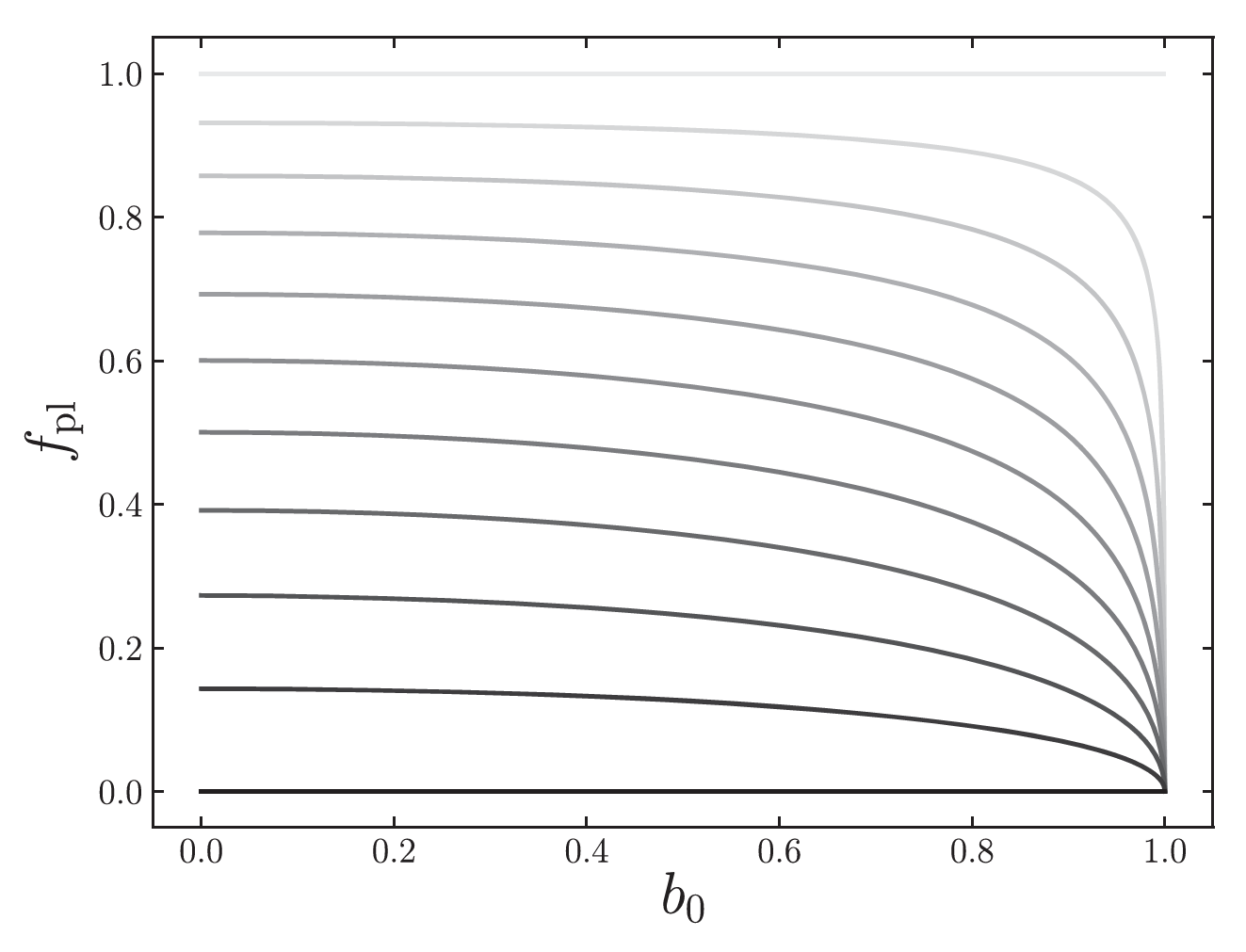
This illustrates several points:
- When \(\Gamma = 0, f_{pl} = 0\), i.e. it is independent of impact parameter when there is no limb darkening;
- With non-zero limb darkening, \(f_{pl}\) is a weak function of \(b_{0}\);
- The range of \(b_{0}\) for which the difference in \(f_{pl}\) is smaller than a given threshold is larger for larger \(\Gamma\), meaning that the lightcurve morphology becomes increasingly degenerate for larger values of \(\Gamma\).
- For \(\Gamma = 1\), only three observables can be measured (\(\Delta F_{max}, t_{c}, f_{ws}\)), but four parameters are required for the model (\(F_{s}, \rho, \beta, t_{*}\)), so all four parameters are degenerate with each other.
However, if the limb darkening parameter is not known, then events must be modeled by considering it to be a free parameter. In this case it can be shown that there is a mathematical one-parameter degeneracy between \(\beta\), \(t_{*}\), \(\Gamma\) and \(F_{s}\rho^{-2}\) such that:
\[\Gamma^{\prime} = \eta \Gamma, \beta^{\prime} = \gamma \beta, t_{*}^{\prime} = \gamma^{-1}t_{*},\] \[\left ( \frac{F_{s}}{\rho^{2}} \right ) = \frac{1}{\eta\gamma}\left ( \frac{F_{s}}{\rho^{2}} \right ),\]where \(\gamma = \frac{1 - \eta\Gamma}{\eta(1 - \Gamma)}\), and \(\eta\) is an arbitrary positive
constant that meets the criteria \(\eta\Gamma \le 1, \gamma\beta \le 1\).
As a result, only the parameters \(F_{s}\) and \(\rho\) are degenerate with each other and \(\Delta F_{max}\) is
constant for fixed values of \((\eta\gamma)^{-1}\).
In the case where \(\rho \gg 1\) but is still finite, \(f_{ws}\) is non-zero, meaning that the peak in the lightcurve has rounded, rather than square, “shoulders”. This fraction gives us an extra observable (\(t_{c}, f_{pl}, f_{ws}\) and \(\Delta F_{max}\)). In this case, there is a continuous mathematical degeneracy such that:
\[\Gamma^{\prime} = \eta\Gamma, \beta^{\prime} = \gamma\beta, t_{*}^{\prime} = \gamma^{-1}t_{*}, \rho^{\prime} = \gamma^{-2}\rho, F_{s}^{\prime} = \eta^{-1}\gamma^{-5}F_{s}.\]Again, \(\eta\) is an arbitrary positive constant meeting the criteria \(\eta\Gamma \le 1, \gamma\beta \le 1\).
In this case, \(F_{s}\) and \(\rho\) become coupled to the larger degeneracy.
Real-world extreme finite source events
While this article explores the theory behind these degeneracies, in practice, not all combinations of parameter values are physically plausible. Extreme finite source events have been detected in the real-world, usually caused by giant or sub-giant source stars. For detailed analysis of these events, see Mróz et al.(2018, 2019, 2020a, 2020b).
References
Chung et al.(2017) Apj, 838, id.154
Gould, A. 1994a ApJ, 421, L71
Han et al.(2019) AJ, 158, 102
Han et al.(2020) AJ, 160, id.64
Johnson et al. (2022), ApJ, 927, 24
Liebes, S. (1964), Phys. Rev. 133, 835
Mróz, P., Ryu, Y.-H., Skowron, J., et al. 2018, AJ, 155, 121
Mróz, P., Udalski, A., et al. 2019, A&A, 622, A201
Mróz, P., Poleski, R., Han, C., et al. 2020, AJ, 159, 262
Mróz, P., Poleski, R., Gould, A., et al. 2020, ApJL, 903,L11
Poleski et al.(2017)
Yoo, J., DePoy, D. L., Gal-Yam, A., et al. (2004), ApJ, 603, 139