Finite source degeneracy
Finite source effects cause measurable distortions only around the peak of a microlensing lightcurve if the angular radius of the source star is comparable with the impact parameter, u0.
Degeneracies can arise if this region in the lightcurve is not well sampled. A good example of this is event OGLE-2015-BLG-1482L analysed in Chung et al.(2017).
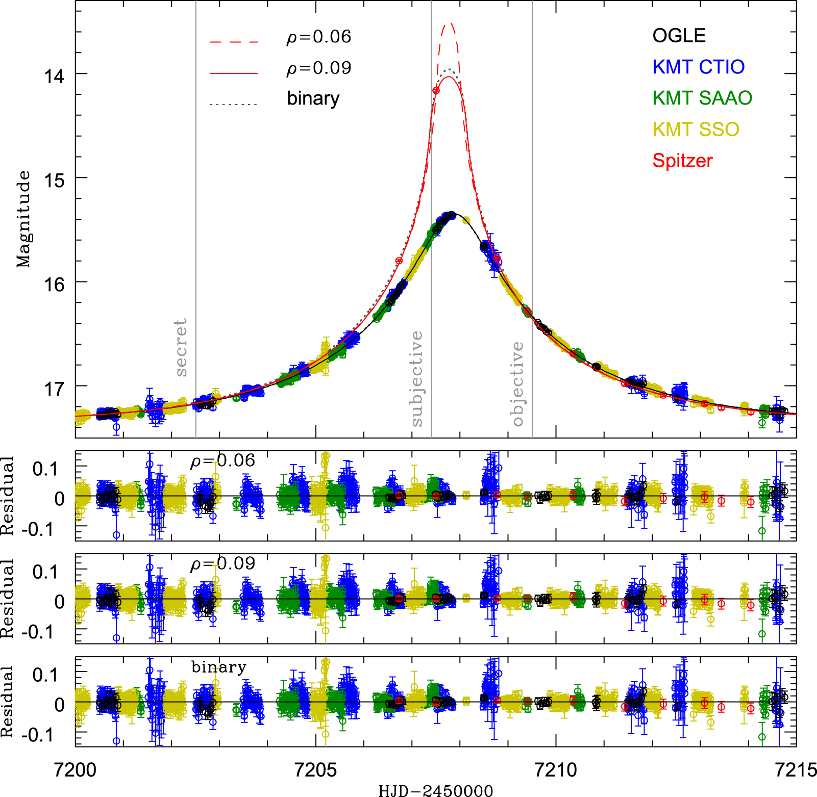
Observations were obtained from both ground-based observatories and the Spitzer Space Telescope for this event. The ground-based lightcurves are well-sampled, but Spitzer obtained ~1 observation per day. The Spitzer lightcurve was sufficient to measure the impact parameter, u, as seen from the spacecraft, as well as the source and blend fluxes, \(f_{s}, f_{b}\). But only one of the Spitzer datapoints was measurably impacted by finite source effects.
For high magnification, point-source, point-lens events, we can state that the magnification \(A_{PSPL} \approx 1/u\). Since \(f_{s}, f_{b}\) are measured, we can infer the (finite-source affected) magnification, \(A_{obs}\) at the time of the one datapoint near the peak using the measured flux F, of that point:
\[A_{obs} = \frac{F - f_{b}}{f_{s}}.\]The ratio of \(A_{obs}\) and \(A_{PSPL}\) can therefore be measured directly from the lightcurve, as shown by Gould (1994):
\[B(z) \equiv \frac{A_{obs}}{A_{PSPL}} \approx A_{obs} u,\]where \(z \equiv u/\rho\). Gould (1994) showed that B(z) reaches a maximum of \(1.34^{2}\) when z~0.91. Inverting a measurement of B(z), there is one solution of z for \(B_{obs} \lt 1\), two solutions for \(1 \lt B_{obs} \lt 1.34\) and no solutions for \(B_{obs} \gt 1.34\).
In the case of Spitzer’s lightcurve for OGLE-2015-BLG-1482L, the one datapoint near the peak has \(A_{obs}\)=1.14 and u=0.06, giving B(z)=1.15, and hence two solutions for z.
For binary events, the finite source degeneracy can result in ambiguous values of the binary separation, s, and mass radio, q. A good example of this is the event KMT-2019-BLG-1339L, analysed by Han et al.(2020).
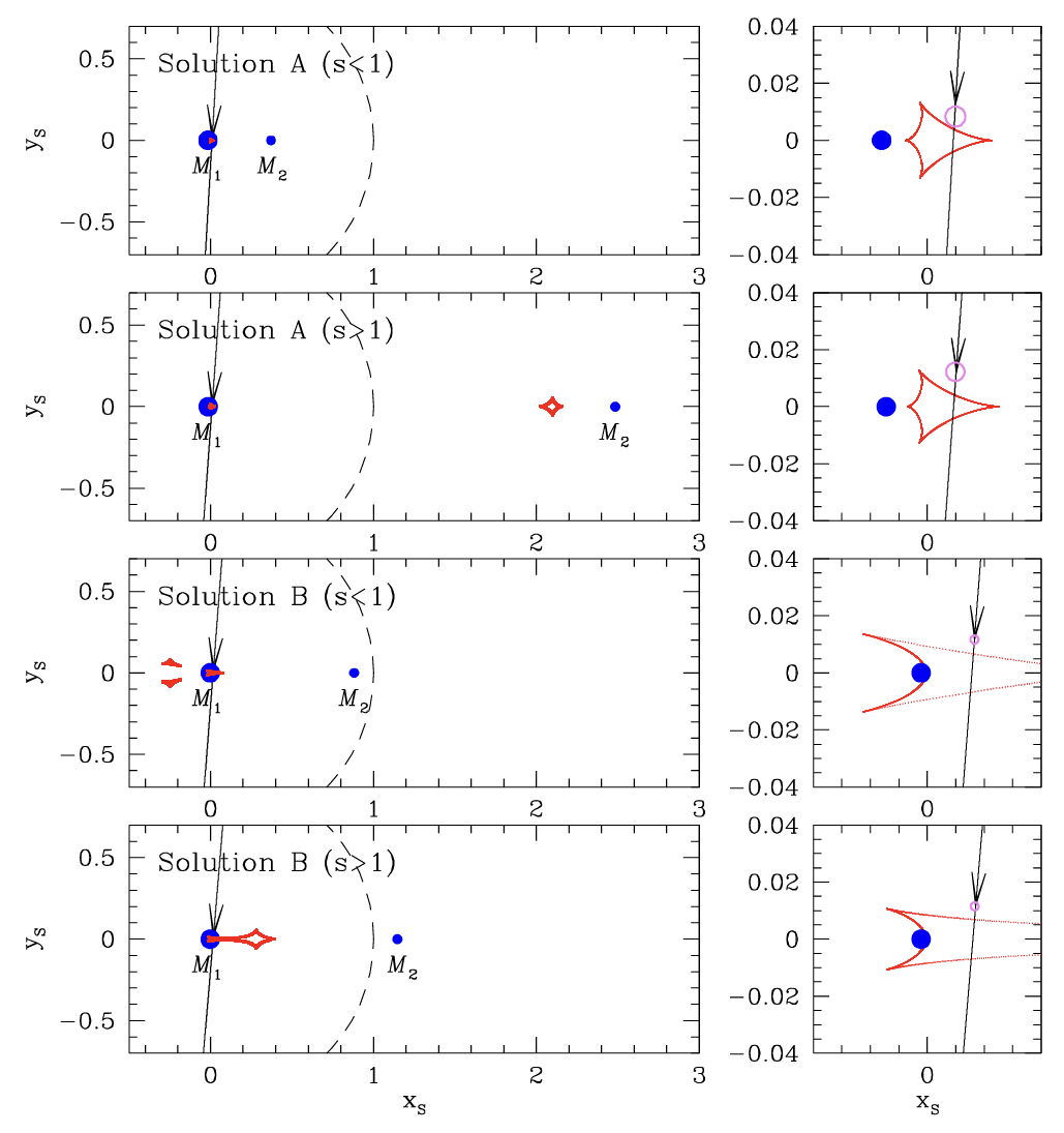
Here, different binary lens separations and mass ratios combine with different source sizes to produce similar lightcurves. These could be distinguished with higher resolution data, but this isn’t always available.
References
Chung et al.(2017) Apj, 838, id.154
Gould, A. 1994a ApJ, 421, L71
Han et al.(2020) AJ, 160, id.64